Fast Calorimeter Simulation Challenge 2022

Welcome to the home of the first-ever Fast Calorimeter Simulation Challenge!

The purpose of this challenge is to spur the development and benchmarking of fast and high-fidelity calorimeter shower generation using deep learning methods. Currently, generating calorimeter showers of interacting particles (electrons, photons, pions, ...) using GEANT4 is a major computational bottleneck at the LHC, and it is forecast to overwhelm the computing budget of the LHC experiments in the near future. Therefore there is an urgent need to develop GEANT4 emulators that are both fast (computationally lightweight) and accurate. The LHC collaborations have been developing fast simulation methods for some time, and the hope of this challenge is to directly compare new deep learning approaches on common benchmarks. It is expected that participants will make use of cutting-edge techniques in generative modeling with deep learning, e.g. GANs, VAEs and normalizing flows.

This challenge is modeled after two previous, highly successful data challenges in HEP – the top tagging community challenge and the LHC Olympics 2020 anomaly detection challenge.

Datasets

The challenge offers three datasets, ranging in difficulty from easy to medium to hard. The difficulty is set by the dimensionality of the calorimeter showers (the number layers and the number of voxels in each layer).

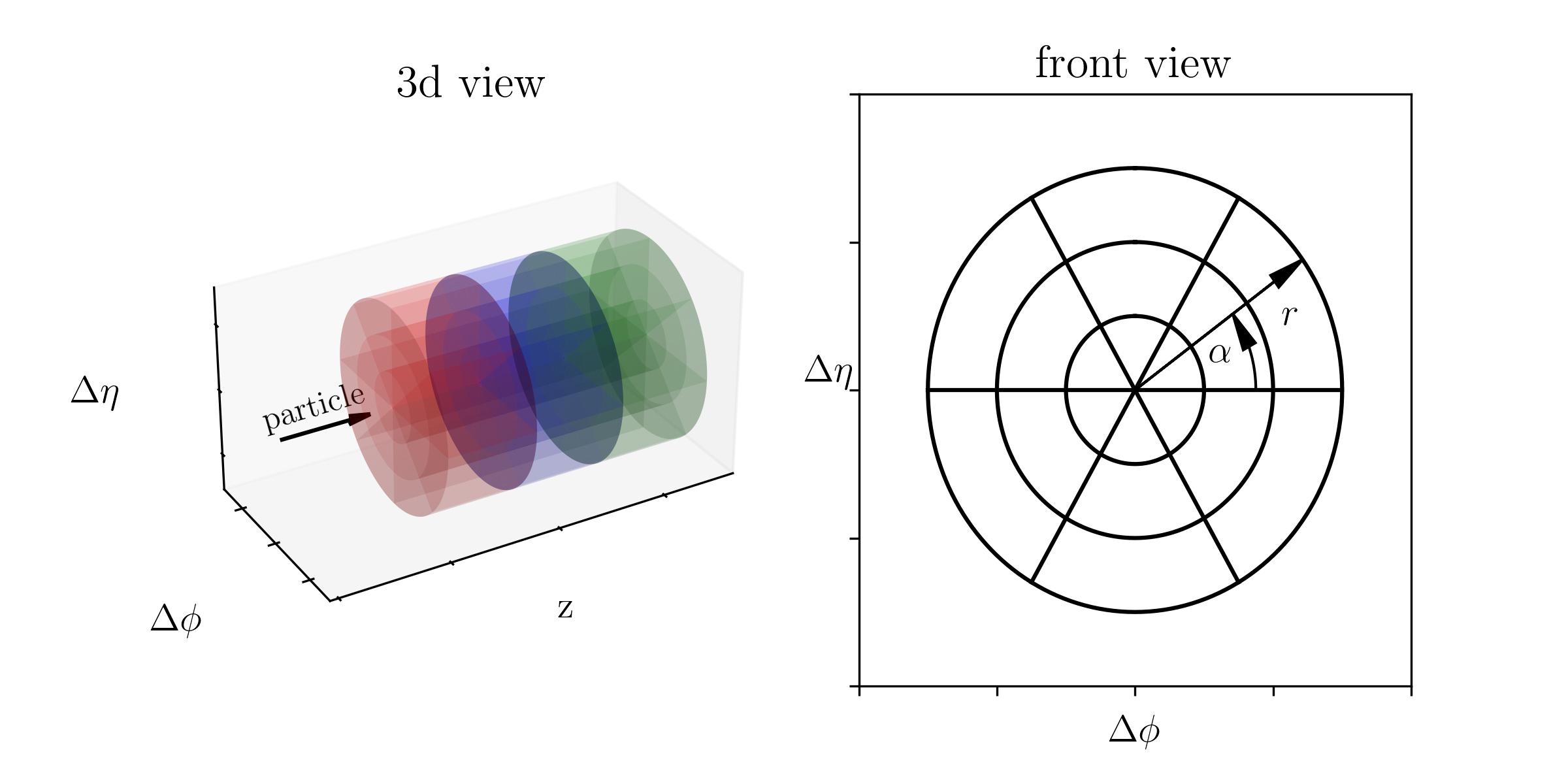
Each dataset has the same general format. The detector geometry consists of concentric cylinders with particles propagating along the z-axis. The detector is segmented along the z-axis into discrete layers. Each layer has bins along the radial direction and some of them have bins in the angle α. The number of layers and the number of bins in r and α is stored in the binning .xml files and will be read out by the HighLevelFeatures class of helper functions. The coordinates Δφ and Δη correspond to the x- and y axis of the cylindrical coordinates. The image below shows a 3d view of a geometry with 3 layers, with each layer having 3 bins in radial and 6 bins in angular direction. The right image shows the front view of the geometry, as seen along the z axis.

Each CaloChallenge dataset comes as one or more .hdf5 files that were written with python's h5py module using gzip compression. Within each file, there are two hdf5-datasets: incident_energies has the shape (num_events, 1) and contains the energy of the incoming particle in MeV, showers has the shape (num_events, num_voxels) and stores the showers, where the energy depositions of each voxel (in MeV) are flattened. The mapping of array index to voxel location is done at the order (radial bins, angular bins, layer), so the first entries correspond to the radial bins of the first angular slice in the first layer. Then, the radial bins of the next angular slice of the first layer follow, ... The shape (num_events, num_z, num_alpha, num_r) can be restored with the numpy.reshape(num_events, num_z, num_alpha, num_r) function.

Dataset 1 can be downloaded from Zenodo with DOI 10.5281/zenodo.8099322. It is based on the ATLAS GEANT4 open datasets that were published here. There are four files, two for photons and two for charged pions. Each dataset contains the voxelised shower information obtained from single particles produced at the calorimeter surface in the η range (0.2-0.25) and simulated in the ATLAS detector. There are 15 incident energies from 256 MeV up to 4 TeV produced in powers of two. 10k events are available in each sample with the exception of those at higher energies that have a lower statistics. These samples were used to train the corresponding two GANs presented in the AtlFast3 paper SIMU-2018-04 and in the FastCaloGAN note ATL-SOFT-PUB-2020-006. The number of radial and angular bins varies from layer to layer and is also different for photons and pions, resulting in 368 voxels (in 5 layers) for photons and 533 (in 7 layers) for pions.
Dataset 2 can be downloaded from Zenodo with DOI 10.5281/zenodo.6366270. It consists of two files with 100k GEANT4-simulated showers of electrons each with energies sampled from a log-uniform distribution ranging from 1 GeV to 1 TeV. The detector has a concentric cylinder geometry with 45 layers, where each layer consists of active (silicon) and passive (tungsten) material. Each layer has 144 readout cells, 9 in radial and 16 in angular direction, yielding a total of 45x16x9 = 6480 voxels. One of file should be used for training the generative model, the other one serves as reference file in evaluation.
Dataset 3 can be downloaded from Zenodo with DOI 10.5281/zenodo.6366323. It consists of 4 files, each one contains 50k GEANT4-simulated eletron showers with energies sampled from a log-uniform distribution ranging from 1 GeV to 1 TeV. The detector geometry is similar to dataset 2, but has a much higher granularity. Each of the 45 layer has now 18 radial and 50 angular bins, totalling 45x50x18=40500 voxels. This dataset was produced using the Par04 Geant4 example. Two of the files should be used for training the generative model, the other two serve as reference files in evaluation.

Datasets 2 and 3 are simulated with the same physical detector which is composed of concentric cylinders, with 90 layers of absorber and sensitive (active) material, which is Tungsten (W) and Silicon (Si), respectively. The thickness of each sub-layer is 1.4mm of W and 0.3 mm of Si, so the total detector depth is 153 mm. The inner radius of the detector is 80 cm.
Readout segmentation is done relevant to the direction of the particle entering the calorimeter. The direction of the particle determines the z-axis of the cylindrical coordinate system, and the entrance position in the calorimeter is (0,0,0). Voxels (readout cells) have the same size in z for both datasets 2 and 3, and they differ in terms of the segmentation in radius (r) and in angle (α).
For z-axis the size of the voxel is 3.4 mm, which corresponds to two physical layers (W-Si-W-Si), and taking into account only the absorber value of radiation length (X0(W)=3.504mm) it makes the z-cell size corresponding to 2*1.4mm/3.504mm = 0.8 X0. In radius the size of the cells is 2.325 mm for dataset 3 and 4.65 mm for dataset 2, which in approximation, taking the Moliere radius of W only, is 0.25 RM for dataset 3 and 0.5 for dataset 2. In α we have 50 cells for dataset 3 and 16 cells for dataset 2, making the size 2π/50 and 2π/16.
The energy threshold for the readout per voxel in datasets 2 and 3 is 15.15 keV.

Files containing the detector binning information for each dataset as well as Python scripts that load them can be found on our Github page. This Jupyter notebook shows how each dataset can be loaded, how the helper class is initialized with the binning.xml files, how high-level features can be computed, and how showers can be visualized. Further high-level features and histograms might be added in the next weeks.

Metrics

The overarching goal of the challenge is to train a generative model on the datasets provided and learn to sample from the conditional probability distribution p(x|E), where x are the voxel energy deposits and E is the incident energy.

Participants will be scored using a variety of metrics. We will include more detailed descriptions of them in the coming months. Metrics will include:

A binary classifier trained on truth GEANT4 vs. generated shower images.
A binary classifier trained on a set of high-level features (like layer energies, shower shape variables).
A chi-squared type measure derived from histogram differences of high-level features.
Training time, calorimeter shower generation time and memory usage.
Interpolation capabilities: leave out one energy in training and generate samples at that energy after training.

It is expected that there will not necessarily be a single clear winner, but different methods will have their pros and cons.

A script to perform the evaluation is available on the Github page. More options will be added in the near future.

In order to run the evaluation, the generated showers should be saved in the same format inside a .hdf5 file as the training showers. Such a file can be created with


import h5py
dataset_file = h5py.File('your_output_dataset_name.hdf5', 'w')
dataset_file.create_dataset('incident_energies',
			    data=your_energies.reshape(len(your_energies), -1),
			    compression='gzip')
dataset_file.create_dataset('showers',
			    data=your_showers.reshape(len(your_showers), -1),
			    compression='gzip')
dataset_file.close()

Note that the distribution of incident energies of the samples should match the distribution in the validation data, as the histograms might otherwise be distorted.

Timeline and Workshop

We will conclude the challenge with a workshop at the end of May 2023 in Rome. There, we will discuss the different approaches, as well as their merits and limits. If you have a contribution, please submit your abstract by May 1st 2023 on the workshop indico page. You will be contacted with instructions to submit your generated samples and the models. The challenge will culminate in a community paper documenting the various approaches and their outcomes.

Please do not hesitate to ask questions: we will use the ML4Jets slack channel to discuss technical questions related to this challenge. You are also encouraged to sign up for the Google groups mailing list for infrequent announcements and communications.

Good luck!

Michele Faucci Giannelli, Gregor Kasieczka, Claudius Krause, Ben Nachman, Dalila Salamani, David Shih and Anna Zaborowska